The article title rather ruins the surprise, but MTF Mapper now supports the measurement of Chromatic Aberration (CA). For now, the emphasis is on the measurement of lateral CA, and in this post I will demonstrate the accuracy of MTF Mapper's implementation, and I will also provide some usage examples.
Before we jump in, I'd just like to point out that I now accept donations to support the development of MTF Mapper through PayPal:
It goes without saying that MTF Mapper remains free and Open Source. There is no obligation to send me money if you use MTF Mapper, and I will continue to add new features to MTF Mapper regardless.
Ok, back to the topic. This post is quite long, so you can skip ahead to the part that interests you if you like. First, I have a review of the concept of lateral chromatic aberration, so you can skip over this to an explanation of how lateral CA is measured in MTF Mapper. Or you can skip to the MTF Mapper CA measurement accuracy experiments and results. Lastly, you can go straight to the usage example if you want to see how to use this, and what the output looks like.
Edge orientation convention
In order to fully explain lateral CA measurement as implemented in MTF Mapper, it is necessary to agree on some convention to describe the orientation of an edge. In this context, "edge" refers to the edge of a trapezoidal slanted-edge target. A radial edge falls along a line passing through the centre of the lens, as seen from the front of the lens. The midpoint of a tangential edge is tangent to a circle concentric with the optical axis of the lens.
 |
| Fig 1: Edge orientation convention |
Although these definitions are strict, we will allow for some deviation from the exact radial and tangential orientations in practice when performing measurements.
Longitudinal Chromatic aberration
Longitudinal Chromatic Aberration (LoCA) appears when a lens does not focus light with different wavelengths at the same focus plane. For example, blue light might be focused slightly in front of the sensor at the same time that green light is perfectly focused on the sensor.
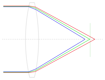 |
| Fig 2: Illustration of longitudinal CA |
If you are capturing an image of a crisp step edge (like we often see in slanted-edge MTF measurements), then the image of the edge in the blue wavelengths still lines up perfectly with the image of the edge in the green wavelengths, it might just be slightly softer because it is out of focus. As you might imagine, LoCA does not necessarily have any preferential direction, i.e., edges in a tangential orientation could be affected by LoCA in exactly the same way as edges with a radial orientation. Of course, things are never quite this simple, so tangential and radial LoCA might be different if your lens suffers from severe astigmatism. Fig 3 gives you some idea of what longitudinal CA could look like in practice.
 |
| Fig 3: Example of simulated longitudinal CA |
For another excellent discussion of CA, including a demonstration of how MTF50 varies with focus position between the three colour channels, you should head over to Jack Hogan's article on the topic, and I should mention that Jack used Jim Kasson's data in places.
Lateral Chromatic aberration
Lateral Chromatic Aberration simply means that the image magnification is dependent on the wavelength. In other words, we might have a lens that can keep blue, green and red wavelengths all concurrently in focus at the sensor (where "in focus" means focus is within some tolerance), but the blue wavelengths are projected with a magnification of 0.99 relative to the green wavelengths, and the red wavelengths with a magnification of 1.01, for example.
 |
| Fig 4: Illustration of lateral CA |
Returning to our slanted-edge target, which we can pretend is located near the edge of the image with a tangential orientation, we will see that the red, green and blue channels have comparable sharpness, but that the edge in the blue channel appears to be shifted inwards towards the centre of the image, and the red channel edge appears to be shifted outwards, relative to the green edge. Keep in mind that this is just one example of how the magnification varies by wavelength, and that other combinations are possible, e.g., both red and blue could have sub-unity magnification. Fig 5 presents a simulated example of lateral CA:
 |
| Fig 5: Example of simulated lateral CA |
So what about radially oriented edges? Well, because the wavelength-depended magnification is radial, we tend to not see any red or blue channel shift at all on radial edges. You could still see some longitudinal CA on those edges, though.
How do you measure CA
Well, I do not know how other people measure it, but MTF Mapper uses the Line Spread Function (LSF) of slanted-edge targets to measure the apparent shift between the red-green and green-blue channel pairs. This means that I first extract an Edge Spread Function (ESF) for each channel, using the tried-and-tested code in MTF Mapper that already compensates for geometric lens distortion. Taking the derivative of the ESF yields the LSF, and the weighted centroid of the LSF is a fairly good estimate of the sub-pixel location of the edge. Rinse and repeat for all three colour channels, and you can estimate CA by subtracting the green channel centroid from the red and blue channel centroids.
I suppose there are many other ways to implement this, really any method that is typically used to perform dense image co-registration will work. Personally, I have played with some Fourier cross-correlation methods [1], as well as a really cool method [2] that estimates the least-squares optimal FIR filter (convolution filter, if you want to sound more hip) to reconstruct the moving image from the fixed image, e.g., estimating the red channel from the green channel, in the CA application case. The centroid of this FIR filter will give you an accurate estimate of the sub-pixel shift. Anyhow, these methods are fine, but there are some advantages to the LSF-based method. The first two that come to mind is that the LSF-based method is not affected by lens distortion, and that you can apply it directly to a Bayer-mosaiced image without requiring a demosaicing algorithm. Just like MTF/SFR measurements, if you are interested in measuring the lens properties, then capturing a raw image and processing the Bayer-mosaiced image directly is the way to go.
Note that the LSF-centroid method I described above can be applied to any edge orientation that is suitable for slanted-edge measurements, so more-or-less anything but integer multiples of 45°. I started out measuring the CA on all edges, but I eventually decided to discard the measurements obtained from radial edges (more precisely, edges that are within 45 degrees of being radially oriented), mostly because I did not know what I was measuring. You can get around this MTF Mapper restriction at the moment by cropping out a single slanted edge, and using the --single-roi MTF Mapper option, which will measure CA regardless of the radial / tangential nature of the edge.
Experimental set-up
To test the accuracy of MTF Mapper's CA measurement functionality, I generated synthetic images with simulated CA. The following three aspects could affect the measurements:
- The magnitude of the shift between the colour channels. Just to make sure that we can detect both subtle and severe CA.
- The apparent sharpness of the edge, since a softer simulated lens yields an image with a more blurry edges. Intuitively, a more blurry edge make the exact location of the edge less well defined, which should increase the uncertainty in the CA measurement.
- Simulated noise, using a realistic sensor noise model (FPN, read noise and photon shot noise), but with a tunable overall SNR. Again, one would expect higher noise levels to increase the uncertainty of the CA measurement.
Some combinations of the above dimensions will now be investigated.
Results: blur vs. noise at a fixed shift, full density RGB
Although one would expect the absolute shift between, say, the red and
the green channels to increase as a function of radial distance, with
worse lateral CA at the edge of the image, this does not make the best
candidate for low-level accuracy evaluation. My first set of experiments
simulated a constant radial shift of 1 pixel between the red and the
green channels across the entire simulated image (and a -1 shift for
blue). This yields 322 usable radial edge measurements from one
simulated "lensgrid" chart image, with most edges ending up with a length between 100 and 120 pixels (this is relevant when discussing the impact of noise). This is what the synthetic image looks like, if you are curious:

The simulated system was similar to my usual
diffraction + square photosite with a simulated aperture of f/4, and a
photosite pitch of 4.73 micron. This time, however, I further employed the "-p
wavefront-box" option to simulate varying degrees of defocus, sweeping
the W020 term from 0λ
through to 3.5λ. Such a range of simulated defocus yields images with
MTF50 values in the range 0.47 to 0.05 cycles per pixel, covering the
range you are likely to encounter in actual use.
 |
| Fig 6: 95th percentile shift error (pixels), full density RGB input images |
In Fig 6 we can see the 95th percentile of the absolute error in the measured shift, relative to the expected shift, as we vary the edge sharpness and the noise level. To put things in perspective, keep in mind that an SNR of 10 is quite poor, and that you should be able to achieve an SNR of 100 with a printed paper test chart without too much effort. Of course, one has to keep in mind that vignetting can be a problem in the image corners: an SNR of 100 in the image centre with about 3.3 stops of vignetting will result in an SNR of 10 in the image corners. Anyhow, this is what the MTF50=0.05, SNR=5 case, with red shifted +1 pixels, and blue shifted -1 pixels looks like:
 |
| Fig 7: An example of what a 1-pixel lateral shift in the red and blue channels looks like under MTF50=0.05 with SNR=5 conditions |
As I will demonstrate later, the measured CA shift values are completely unbiased. Here I show the 95th percentile of the error, but the mean value in each cell (over all 322 edges) deviates less than 0.013 pixels from the expected value in all cells, including the worst-case combination of blur and noise. One minor detail remains, though: the results in Fig 6 were obtained with full density RGB input images, meaning the simulation generated individual R, G and B values at each pixel, so this is representative of a Foveon-like sensor, not a typical Bayer CFA sensor.
Results: blur vs. noise at a fixed shift, Bayer-mosaiced
A more representative example would be to reduce the full-density RGB image to a Bayer-mosaiced image, and then processing the resulting image as using MTF Mapper's "--bayer green" input option. This will cause the CA measurements to be performed using the mosaiced data; note that the "--bayer green" option will still cause MTF Mapper to use the appropriate red and green Bayer subsets for CA measurements, and that only the MTF data will be extracted using only the green Bayer subset. Since the number of samples along each edge is reduce by the Bayer mosaicing, we expect an increase in the CA measurement error.
 |
| Fig 8: 95th percentile shift error (pixels), Bayer mosaic input images |
Comparing Fig 8 to Fig 6 reveals that we now require better SNR values to maintain the same level of accuracy in the CA shift measurements. For example, the SNR=40 column in Fig 8 is a reasonable match for the SNR=20 column in Fig 6. Ok, perhaps Bayer-mosaiced SNR=40 is slightly better than full-RGB SNR=20, but you get the idea.
Results: blur vs. noise at a fixed shift, Bayer demosaiced
What happens if we take the Bayer-mosaiced images generated in the previous step, and we run them through a demosaicing algorithm to produce another full-density RGB image? I chose to use OpenCV's built-in demosaicing algorithm, COLOR_BayerRG2BGR_EA. This may not be the best demosaicing algorithm on the planet, but it produced output that was consistent. |
| Fig 9: 95th percentile shift error (pixels), demosaiced input images |
Comparing Fig 9 to Fig 8 delivers a few surprises: At the SNR=100 and SNR=50 noise levels, the demosaiced image produced slightly more accurate results around the MTF50=0.24 scenario rather than at the sharpest setting (MTF50=0.47), and the demosaiced image actually performed slightly better than the raw Bayer-mosaiced case in the high-blur, low-SNR corner.
In retrospect, it makes sense that the demosaiced CA measurement is less accurate on very sharp edges, because aliasing is likely to make demosaicing harder, or less accurate, perhaps. The other surprise is perhaps also not so unexpected, since demosaicing is an interpolation process, thus we expect it to filter out high-frequency noise to some extent. In the lower-right corner of our table we encounter scenarios where there is little high-frequency content to the edge location (the edge is blurry, after all), but we have a lot of noise, so some additional low-pass filtering courtesy of the demosaicing interpolation helps just enough. Perhaps this is an indication that MTF Mapper could benefit from applying additional smoothing during low-SNR CA measurements in future.
Results: shift vs. noise at a fixed blur, Bayer-mosaiced
Note that I will now skip over the full-density RGB results for brevity, and move right along to raw Bayer-mosaiced results obtained at different simulated lateral CA shifts. The expectation is that the shift measurement accuracy should be independent of the actual shift magnitude within the usable measurement range, which is probably around ±20 pixels. Only two noise levels were investigated, SNR=50 and SNR=10, representing the good-but-not-perfect, and need-to-improve-lighting scenarios. |
| Fig 10: Difference between measured CA shift and expected CA shift, low noise scenario, raw mosaiced image |
 |
| Fig 11: Difference between measured CA shift and expected CA shift, high noise scenario, raw mosaiced image |
The boxplots not only give us an indication of the spread of the CA shift measurements, but also hint at the smallest difference in shift that can be discerned. As shown in Fig 10, MTF Mapper can easily measure differences in CA shift of well below 0.1 pixels under good SNR conditions, but Fig 11 shows that there is some overlap between adjacent shift steps under very noisy conditions. By overlap I mean that adjacent boxes are separated by an expected difference of 0.1 pixels in CA shift, but we can see that the height of the whiskers of the boxes in Fig 11 exceeds 0.1 pixels. Another reassuring feature is that we can see that all the boxes are centred nicely around an error of zero, thus the measurements are unbiased.
Results: shift vs. noise at a fixed blur, Bayer demosaiced
Similar to the previous experiment, but with an additional demosaicing step, again using OpenCV's algorithm. I will only show the noisy case for brevity:
 |
| Fig 12: Difference between measured CA shift and expected CA shift, high noise scenario, OpenCV demosaiced image |
If you compare Figs 11 and 12, you might notice that the spread of the differences is slightly smaller in Fig 12, i.e., just like we observed in Fig 9 we are seeing a small noise reduction benefit with demosaicing, but without adding any bias to the measurement. Well, that is with OpenCV's demosaicing algorithm. I also repreated the experiment using LibRaw's open_bayer() function, but I suspect that I am doing something wrong, because I get some pronounced zippering artifacts, and this boxplot:
 |
| Fig 13: Difference between measured CA shift and expected CA shift, low noise scenario, LibRaw AHD demosaic image |
Unlike all the other scenarios, the LibRaw AHD experiment yields CA shift measurements that have a very obvious bias, seen as the systematic deviation from a zero-mean error in Fig 13. I am not going to say much more here, because it is most likely user error on my part.
Recommendations following the experiments
Several aspects that affect the accuracy of lateral CA measurements were considered above, including the magnitude of the shift between channels, the overall sharpness of the edge, and the prevailing signal-to-noise conditions. It is hard to make any recommendation without choosing some arbitrary threshold of when a CA measurement is considered "accurate enough". My rule of thumb in these matters is that an accuracy of 0.1 pixels is a reasonable target, since this figure often appears in machine vision literature. Given this target, we can break down the results above to produce the following recommendations:
- The easiest parameter to control, and the one you should probably put the most effort into controlling, is the signal-to-noise ratio. If your images look like Fig 7 above, you simply cannot expect accurate results. If you can keep the SNR at 30 or higher, you can expect to hit the target accuracy of 0.1 pixels.
- The next parameter you should try to control is focus. CA measurements on well-focused images are more accurate than those obtained from blurry photos. Having said that, some lenses are just not very sharp, and if you have extreme field curvature your image corners are bound to be out of focus. One recommendation here is to capture two shots: one with the "optimal" focus (whatever your criteria for that are), and another obtained after focusing in one of the image corners. This two-photo strategy is really only necessary in extreme cases when you face blurry corners and extreme vignetting, or you could not control the SNR because of external factors.
- Do not measure CA on demosaiced images if you can help it. For Fuji X-trans you have no choice with MTF Mapper at the moment, but for any Bayer CFA layout you should use raw images when possible. At some point, I will look at other demosaicing algorithms, maybe even LightRoom, just to see what is possible.
User interface and visualization
CA measurements are now available through the MTF Mapper GUI. If you are new to MTF Mapper, you can view the user guide after installation (e.g., using this link to install the Windows 10 binaries) under the help menu in the GUI, or you can download a PDF version from this link if you want to browse through the guide first before you decide to install MTF Mapper.
 |
| Fig 14: Preferences dialogue |
As shown in Fig 14, MTF Mapper now has a new output type (a), as well as an option to control which type of visualization to generate (b). The CA measurement is visualized either as the actual shift in pixels (or microns, if you set the pixel size and select the "lp/mm units" option), measured in the red/blue channels, or the shift can be expressed as a percentage of the radial distance from the measurement to the centre of the image. I processed some images of my Sigma 10-20 mm lens on a Nikon D7000 to illustrate:
 |
| Fig 15: lateral CA map, with shift indicated in pixels |
 |
| Fig 16: same lateral CA map, but this time the shift is expressed as a fraction of the radial distance |
Personally, I prefer the visualization in Fig 15, but I have noticed that other software suites offer the visualization in Fig 16; normalizing the lateral CA shift by the radial distance should help to make the measurement less dependent on the final print size, I suppose. The main problem with the way that I have implemented this method (Fig 16) is that there is an asymptote at the centre of the lens where the radial distance is very small. This rather ruins the scaling of the plot; I think Imatest works around this problem by suppressing the central 30% of the plot. I should probably do something similar, but suggestions are welcome.
Here is a crop of a target trapezoid from the top-left corner of the image, with a measured red channel shift of -0.4 (i.e, red is smaller than green), and a measured blue channel shift of -1.06 on the upper left edge, which gives it the green tinge we see in Fig 17. The opposite edge sports a magenta tinge, as we would expect.
 |
| Fig 17: Crop of a target from the top-left corner of the chart image used to produce Figs 15 and 16. Please excuse the sad condition of the test chart I used here :) |
For my usage patterns, I think it would be very helpful to be able to select a specific edge, and have MTF Mapper display the lateral CA measurement for that edge. My plan is to add the CA measurement to the info display what goes with the MTF/SFR curve plot that pops up when you click on an edge in the Annotated image output. In the meantime, both the smoothed, gridded data and the raw measurements are made available for your enjoyment.
If you are a command-line user, you can enable CA measurement with the "--ca" flag. The raw CA measurements are available in a self-documenting file called "chromatic_aberration.txt" in the output directory, but you also get the plot as "ca_image.png". Note that GUI users can now also get their hands on both these files by using the "Save all results" button on the main GUI window after completing a run.
Lastly, I should emphasize that it is important to achieve good alignment between the sensor and the test chart for CA measurements. I think that there might be some tilt in my results shown in Figs 15 and 16 above. Or perhaps lateral CA is not supposed to be perfectly symmetric; come to think of it, I suppose it would be affected by tilted lens elements, for example. At any rate, you can use MTF Mapper's built-in Chart Orientation output mode to help you refine your chart alignment.
Conclusion
You can try out the latest version of MTF Mapper yourself to play with the new features. I have released Windows binaries of version 0.7.29, and I will probably release some Ubuntu .debs as well soon. Or you can build from source :)
In future, I plan on doing some comparisons with other related tools, probably Imatest and QuickMTF, to see how well they perform on my synthetic images. And I hope to understand the problems I have run into with certain demosaicing algorithms, although I still think that lateral CA measurements should be performed on raw images whenever possible.
References
- Almonacid-Caballer, Jaime, Josep E. Pardo-Pascual, and Luis A. Ruiz. "Evaluating Fourier cross-correlation sub-pixel registration in Landsat images." Remote Sensing 9, no. 10 (2017): 1051.
- Gilman, Andrew, Leist, Arno, "Global Illumination-Invariant Fast Sub-Pixel Image Registration." The Eighth International Multi-Conference on Computing in the Global Information Technology (ICCGI), Nice, France, (2013):95-100.